T. Andrew Yang: CSCI5333

CSCI 5333 Data Base Management System

Spring 2002 (1/14-5/6)

Chapter 15: Further Dependencies & Higher Normal Forms

15.1.1 Relation Decomposition and Insufficiency of Normal Forms

Looking at an individual relation to test whether it is in a higher normal form does not, on its own, guarantee a good design; rather, a set of relations that together form the relational database schema must possess certain additional properties to ensure a good design.

The dependency preservation property and the lossless (or nonadditive) join property .

A single universal relation schema R = {A1, A2, ..., An} that includes all the attributes of the database .

A decomposition of R: D = {R1, R2, R3, ..., Rm}.

The attribute preservation condition of a decomposition: Each attribute in R will appear in at least one relation schema in the decomposition so that no attributes are "lost".

NOTE: Having each individual relation R_i in the decomposition D to be in BCNF (or 3NF) may not be sufficient to guarantee a good database design on its own.

Problem: Spurious tuples out of a natural join. Example: See Fig. 14.6.

15.1.2 Decomposition and Dependency Preservation

The dependency preservation condition (informal definition): Each functional dependency f specified in F either appears directly in one of the relation schemas R_i in the decomposition D or could be inferred from the dependencies that appear in some R_i.

Formal definition:

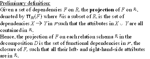
Exercise: Examine Fig. 14.12(a) and produce the projection of F on Lots1Ax. Repeat the same process on Lots1Ay.

An example of a decomposition that does not preserve dependencies: Figure 14.12(a).

Exercise: Verify the above statement.

Another example: Figure 14.13 with any of the three alternative decompositions

Alternative 1: {STUDENT, INSTRUCTOR} and {STUDENT, COURSE}.
Alternative 2: {COURSE, INSTRUCTOR} and {COURSE, STUDENT}
Alternative 3: {INSTRUCTOR, COURSE} and {INSTRUCTOR, STUDENT}.

Exercise: Verify that alternative 1 decomposition is not dependency-preserving, with respect to the original dependencies.

The decompositions in Figure 14.11 are dependency-preserving.

Exercise: Verify the above statement.

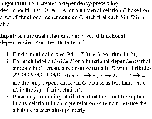
Claim 1: It is always possible to find a dependency-preserving decomposition D with respect to F such that each relation R_i in D is in 3NF. (See Algorithm 15.1)

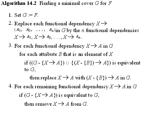
Minimal set of functional dependencies: (from Chapter 14)

Algorithm 14.2

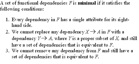
Note: In step 3 of algorithm 14.2, suppose the new set of functional dependencies after removing an attribute B is called G'. Then it is true that G' covers G. So what's left is to show that G covers G'. A 'short cut' approach is to show that the new functional dependency (X - {B]) --> A in G' can be inferred from G.

Exercise 14-21

Another exercise: Apply algorithm 14.2 to find a minimal cover for F = {fd1, fd2, fd3, fd4} as defined for the relation LOTS in Figure 14.11 on page 492.

Let LOTS = (p, c, l, a, pr, t).
Step 1: G = F.
Step 2: G = { p->c; p->l; p->a; p->pr; p->t;
c, l -> p; c, l -> a; c, l -> pr; c, l -> t;
c->t;
a->pr }
Step 3: Remove an attribute from the left hand side (lhs) of the functional dependencies with multiple-attribute lhs, that is, c, l -> p; c, l -> a; c, l -> pr; c, l -> t.. Each such removal will result in a new set of functional dependencies, G'. Since G' always covers G, what is left is to show that G covers G'.
3.a. (Removing attribute c from c, l -> p) Show that l->p can be derived from G. (no)
3.b. (Removing attribute l from c, l -> p) Show that c->p can be derived from G. (no)
3.c. (Removing attribute c from c, l -> a) Show that l->a can be derived from G. (no)
3.d. (Removing attribute l from c, l -> a) Show that c->a can be derived from G. (no)
3.e. (Removing attribute c from c, l -> pr) Show that l->pr can be derived from G. (no)
3.f. (Removing attribute l from c, l -> pr) Show that c->pr can be derived from G. (no)
3.g. (Removing attribute c from c, l -> t) Show that l->t can be derived from G. (no)
3.h. (Removing attribute l from c, l -> t) Show that c->t can be derived from G. (yes!)
So, at the end of step 3,
G = { p->c; p->l; p->a; p->pr; p->t;
c, l -> p; c, l -> a; c, l -> pr; c -> t;
c->t;
a->pr }
Step 4: Check each of the functional dependencies in G to see if it can be removed. Each such removal results in a new set of functional dependencies, G'. Since G always covers G', the job left for us to do is to show that G' covers G.
4.a. Can p->c be removed? (not really!)
4.b. Can p->l be removed? (not really!)
4.c. Can p->a be removed? (not really!)
4.d. Can p->pr be removed? (yes, because p->a and a->pr)
4.e. Can p->t be removed? (yes, because p->c and c->t)
4.f. Can c,l->p be removed? (not really!)
4.g. Can c,l->a be removed? (yes, because c,l->p and p->a)
4.h. Can c,l->pr be removed? (yes, because c,l->p and p->pr)
4.i. Can c->t be removed? (yes, because of redundancy in the set)
4.j. Can c->t be removed? (not really!)
4.k. Can a->pr be removed? (not really!)

So, at the end of step 4,
G = { p->c; p->l; p->a; ~~p->pr; p->t;~~
c, l -> p; c, l -> a; c, l -> pr; c -> t;
c->t;
a->pr }
G = { p->c; p->l; p->a; c, l -> p; c->t; a->pr} is a minimal cover of F.

Algorithm 15.1:

Exercise: Consider the relation schema EMP_DEPT in Figure 14.3(a) and the following set G of functional dependencies on EMP_DEPT: G = {SSN --> {ENAME, BDATE, ADDRESS, DNUMBER}, DNUMBER --> {DNAME, DMGRSSN}}. Decompose EMP_DEPT by applying algorithm 15.1.

Another Exercise: Repeat the exercise by applying the algorithm on EMP_PROJ in Figure 14.3(b).

Algorithm 15.1 is called the relational synthesis algorithm , because each relation schema in the decomposition is synthesized (constructed) from the set of functional dependencies in G with the same left-hand-side X.

Ø Go to the Index

15.1.3 Decomposition and Lossless (Nonadditive) Joins

Nonadditive join property ensures that no spurious tuples are generated when a NATURAL JOIN operation is applied to the relations in the decomposition.

The word loss in lossless refers to loss of information, not to loss of tuples.

The term nonadditive join is preferred.

Algorith 15.2: Testing for the nonadditive join property

Input: A universal relation R, a decomposition of R, and a set F of functional dependencies.

Algorithm 15.2 allows us to test whether a particular decomposition D obeys the lossless join property with respect to a set of functional dependencies F.

Once a row consists only of "a" symbols, we know that the decomposition has the lossless join property, and we can stop applying the functional dependencies (Step 4 of the algorithm) to the matrix S.

An example of testing the algorithm: See Fig. 15.1(a).

Another example: Fig. 15.1 (c).

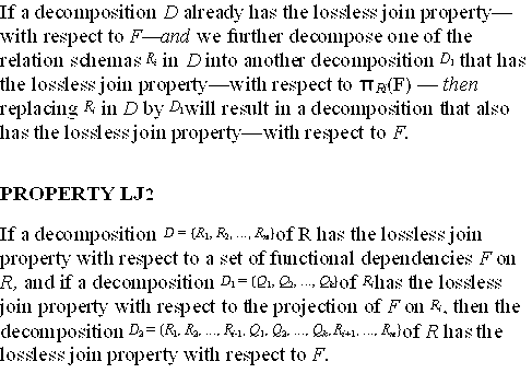
Some properties of lossless join decompositions:

binary decompositions

Exercise: Verify the property by using examples in Section 14.3 and Section 14.4.

p.489: Figure 14.10(b)
p.492: Figure 14.11(a)(b)
p.492: Figure 14.11(b)(c)

The "transitive" property:

Algorithm 15.3: Relational decomposition into BCNF relations with lossless join property

Input: A universal relation R and a set of functional dependencies F on the attributes of R.

Review: Fig. 14.11, 14.12, and 14.13.

Algorithm 15.4: Relational synthesis algorithm with dependency preservation and lossless join property.

Input: A universal relation R and a set of functional dependencies F on the attributes of R.

Outcome: A decomposition D of R that satisfiies the following constraints:
1. Preserves dependencies.
2. Has the lossless join property.
3. Is such that each resulting relation schema in the decomposition is in 3NF.
NOTE: Algorithm 15.4 is a modification of Algorithm 15.1, which, unlike 15.4, does not guarantee the lossless join property.

Exercise: Decompose the TEACH relation on page 495 by applying algorithm 15.4 .

Algorithm 15.4a: Finding a key K for relation schema R based on a set F of functional dependencies.

Exercise: Apply algorithm 15.4a to the EMP_PROJ relation on page 470 to determine the key of the relation.

Another exercise: Exercise 15.24 on page 525.

It is not always possible to find a decomposition into relation schemas that preserves dependencies and allows each relation schema in the decomposition to be in BCNF (instead of 3NF as in Algorithm 15.4). See Fig. 14.12 and 14.13.

Ø Go to the Index

15.1.4 Problems with Null Values and Dangling Tuples

Problems with Null Values:

Problem 1: In general, whenever a relational database schema is designed where two or more relations are interrelated via foreign keys , particular care must be devoted to watching for potential null values in foreign keys. This can cause unexpected loss of information in queries that involve joins on that foreign key.

Example: See Figure 15.2(a)(b)

Problem 2: Effect on built-in functions ?

The "Dangling Tuples" Problem

See Fig. 15.3: Dangling tuples are represented in only one of the two relations that represent employees and hence are lost if we apply a natural join operation.

Ø Go to the Index

15.2 Multivalued Dependencies and Fourth Normal Form

Multivalued dependencies are a consequence of first normal form.

Informally, whenever two independent 1:N relationships A:B and A:C are mixed in the same relation, an MVD may arise.

Example: (See Fig. 15.4, p.515)

ENAME -->> PNAME: An employee may work on multiple projects.
ENAME -->> DNAME: An employee may have multiple dependents.

Question: Can the last two tuples in Fig. 15.4 be removed?

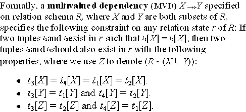
Formal Definition of MVD:

Exercise: Verify that the EMP relation satisfies the above constraints.

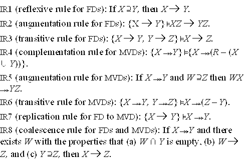
15.2.2 Inference Rules for Functional and Multivalued Dependencies

15.2.3 Fourth Normal Form

An MVD X -->> Y in R is a trivial MVD if either (a) Y is a subset of X, or (b) the union of X and Y equals R.

Exercise: Examine the EMP relation in Fig. 15.4(a) to determine if it is in 3NF, BCNF, and 4NF. Justify your answers.

Problems with relations that are not in 4NF: waste of space + update anomalies

Benefis of 4NF: See the illustration in Fig. 15.5.

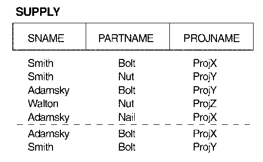
Question: Is the SUPPLY relaiton in Figure 15.4(c) in 4NF? Justify your answer.

NOTE: Relations containing nontrivial MVDs tend to be all key relaitons .

15.2.4 Lossless Join Decomposition into 4NF Relations

Exercise: Verify that the decomposition of EMP into EMP_PROJECTS and EMP_DEPENDENTS (p.515) is a lossless join decomposition.

Algorithm 15.5: Relational decomposition into 4NF relations with lossless join property (modified from algorithm 15.3).

Exercise: Apply algorithm 15.5 to the EMP relation in Fig. 15.4(a).

Ø Go to the Index

15.3 Join Dependencies and Fifth Normal Form

An MVD is a special case of a JD where n = 2.

5NF:

Example: The supplier-part-project relation in Fig. 14.4(c).

Exercise: Examine the above relation to determine why it is not in 5NF.

Decomposition into 5NF relations: See Fig. 14.4(d).

Another exercise: Verify the statement "Applying NATURAL JOIN to any two of these relations produces spurious tuples, but applying NATURAL JOIN to all three together does not."

Ø Go to the Index